A.1 Design Infiltration Rate Steps
For BMPs that are designed to infiltrate, facility size is based upon the design infiltration rate. In order to determine the design infiltration rate, first determine the measured (initial) saturated hydraulic conductivity (Ksat) of the soil. Once the measured saturated hydraulic conductivity is measured, calculation of the design infiltration rate is required.
Methods for determining the initial and design rates are provided below.
A.2 Determining the Measured Saturated Hydraulic Conductivity
Use one of the following three methods to determine the measured saturated hydraulic conductivity. The method used is dependent upon the BMP proposed. Review the design criteria for the BMP proposed to determine which method to use.
A.2.1 Large Scale Pilot Infiltration Test (PIT)
Large-scale in-situ infiltration measurements, using the Pilot Infiltration Test (PIT) described below is the preferred method for estimating the measured (initial) saturated hydraulic conductivity (Ksat) of the soil profile beneath the proposed infiltration facility. The PIT reduces some of the scale errors associated with relatively small-scale double ring infiltrometer or “stove-pipe” infiltration tests. It is not a standard test but rather a practical field procedure recommended by Ecology’s Technical Advisory Committee.
A.2.1.1 Infiltration Test Method and Requirements
Conduct testing between December 1 and April 1.
The horizontal and vertical locations of the test pit shall be surveyed by a Washington State Licensed Land Surveyor with location clearly shown in the Soils Report.
Excavate the test pit to the estimated bottom surface elevation of the proposed infiltration facility where the infiltration facility meets the native soil. If the native soil has to meet subgrade compaction requirements (such as needed for BMP L633 - Permeable Pavements), compact the native soil prior to testing. Lay back the slopes sufficiently to avoid caving and erosion during the test. Alternatively, consider shoring the sides of the test pit.
The horizontal surface area of the bottom of the test pit should be approximately 100 square feet. Accurately document the size and geometry of the test pit.
Install a vertical measuring rod (minimum 5-ft. long) marked in half-inch increments in the center of the pit bottom.
Use a rigid 6-inch diameter pipe with a splash plate on the bottom to convey water to the pit and reduce side-wall erosion or excessive disturbance of the pond bottom. Excessive erosion and bottom disturbance will result in clogging of the infiltration receptor and yield lower than actual infiltration rates.
Add water to the pit at a rate that will maintain a water level between 6 and 12 inches above the bottom of the pit. A rotameter can be used to measure the flowrate into the pit.
Note: The depth should not exceed the proposed maximum depth of water expected in the completed facility. For infiltration facilities serving large contributing areas, designs with multiple feet of standing water can have infiltration tests with greater than 1 foot of standing water.
Every 15-30 min, record the cumulative volume and instantaneous flowrate in gallons per minute necessary to maintain the water level at the same point on the measuring rod.
Keep adding water to the pit until one hour after the flow rate into the pit has stabilized (constant flowrate; a goal of 5% variation or less variation in the total flow) while maintaining the same pond water level. The total of the pre-soak time plus one hour after the flowrate has stabilized should be no less than 6 hours.
After the flowrate has stabilized for at least one hour, turn off the water and record the rate of infiltration (the drop rate of the standing water) in inches per hour from the measuring rod data, until the pit is empty. Consider running this falling head phase of the test several times to estimate the dependency of infiltration rate with head.
At the conclusion of testing, over-excavate the pit to see if the test water is mounded on shallow restrictive layers or if it has continued to flow deep into the subsurface. The depth of over-excavation varies depending on soil type and depth to hydraulic restricting layer, and is determined by the design engineer or certified soils professional. Mounding is an indication that a mounding analysis is necessary.
Calculate and record the saturated hydraulic conductivity rate in inches per hour in 30 minutes or one-hour increments until one hour after the flow has stabilized.
Note: Use statistical/trend analysis to obtain the hourly flowrate when the flow stabilizes. This would be the lowest hourly flowrate.
A.2.2 Small Scale Pilot Infiltration Test (PIT)
Use the same procedure as used for the Large Scale Pilot Infiltration Test with the following changes:
The horizontal surface area of the bottom of the test pit should be 12 to 32 square feet. It may be circular or rectangular, but accurately document the size and geometry of the test pit.
The rigid pipe with splash plate may be a 3 inch diameter pipe for pits on the smaller end of the recommended surface area, and a 4 inch pipe for pits on the larger end of the recommended surface area.
Pre-soak period: Add water to the pit so that there is standing water for at least 6 hours. Maintain the pre-soak water level at least 12 inches above the bottom of the pit.
At the end of the pre-soak period, add water to the pit at a rate that will maintain a 6-12 inch water level above the bottom of the pit over a full hour. The depth should not exceed the proposed maximum depth of water expected in the completed facility.
Every 15 minutes, record the cumulative volume and instantaneous flowrate in gallons per minute necessary to maintain the water level at the same point (between 6 inches and 1 foot) on the measuring rod. The specific depth should be the same as the maximum designed ponding depth (usually 6 – 12 inches).
After one hour, turn off the water and record the rate of infiltration (the drop rate of the standing water) in inches per hour from the measuring rod data, until the pit is empty.
A self-logging pressure sensor may also be used to determine water depth and drain-down.
At the conclusion of testing, over-excavate the pit to see if the test water is mounded on shallow restrictive layers or if it has continued to flow deep into the subsurface. The depth of excavation varies depending on soil type and depth to hydraulic restricting layer, and is determined by the design engineer or certified soils professional. The soils professional should judge whether a mounding analysis is necessary.
Calculate and record the saturated hydraulic conductivity rate in inches per hour in 30 minute or one-hour increments until one hour after the flow has stabilized.
Note: Use statistical/trend analysis to obtain the hourly flowrate when the flow stabilizes. This would be the lowest hourly flowrate.
A.2.3 Soil Grain Size Analysis Method
The Soil Grain Size Analysis can only be used to determine the initial Ksat if the site has soils unconsolidated by glacial advance.
For each defined layer below the infiltration facility (minimum depth requirements are contained in the design criteria of each BMP) estimate the saturated hydraulic conductivity in cm/sec using the following relationship (see Massmann 2003, and Massmann et al., 2003)

D10, D60 and D90 are the grain sizes in mm for which 10 percent, 60 percent and 90 percent of the sample is more fine
ffines is the fraction of the soil (by weight) that passes the #200 sieve (Ksat is in cm/s).
If the licensed professional conducting the investigation determines that deeper layers will influence the rate of infiltration for the facility, soil layers at greater depths must be considered when assessing the site’s hydraulic conductivity characteristics. Massmann (2003) indicates that where the water table is deep, soil or rock strata up to 100 feet below an infiltration facility can influence the rate of infiltration. Note that only the layers near and above the water table or low permeability zone (e.g., a clay, dense glacial till, or rock layer) need to be considered, as the layers below the groundwater table or low permeability zone do not significantly influence the rate of infiltration. Also note that this equation for estimating hydraulic conductivity assumes minimal compaction consistent with the use of tracked (i.e., low to moderate ground pressure) excavation equipment. If the soil layer being characterized has been exposed to heavy compaction, the hydraulic conductivity for the layer could be approximately an order of magnitude less than what would be estimated based on grain size characteristics alone (Pitt, 2003). In such cases, compaction effects must be taken into account when estimating hydraulic conductivity. For clean, uniformly graded sands and gravels, the reduction in Ksat due to compaction will be much less than an order of magnitude. For well-graded sands and gravels with moderate to high silt content, the reduction in Ksat will be close to an order of magnitude. For soils that contain clay, the reduction in Ksat could be greater than an order of magnitude.
If greater certainty is desired, the in-situ saturated conductivity of a specific layer can be obtained through the use of a pilot infiltration test (PIT).
Once the saturated hydraulic conductivity for each layer has been identified, determine the effective average saturated hydraulic conductivity below the facility. Hydraulic conductivity estimates from different layers can be combined using the harmonic mean.
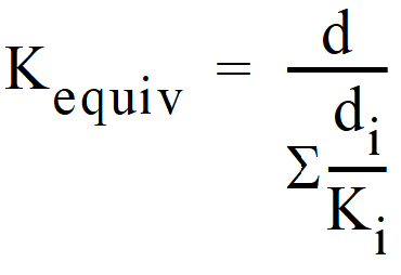
d = total depth of the soil column
di = thickness of layer “i” in the soil column
Ki = saturated hydraulic conductivity of layer “i” in the soil column.
The depth of the soil column, d, typically would include all layers between the facility bottom and the water table. However, for sites with very deep water tables (>100 feet) where groundwater mounding to the base of the facility is not likely to occur, it is recommended that the total depth of the soil column in (Equation 4 - 52) be limited to approximately 20 times the depth of facility, but not more than 50 ft. This is to ensure that the most important and relevant layers are included in the hydraulic conductivity calculations. Deep layers that are not likely to affect the infiltration rate near the facility bottom should not be included in (Equation 4 - 52). (Equation 4 - 52) may over-estimate the effective hydraulic conductivity value at sites with low conductivity layers immediately beneath the infiltration facility. For sites where the lowest conductivity layer is within five feet of the base of the pond, it is suggested that this lowest hydraulic conductivity value be used as the equivalent hydraulic conductivity rather than the value from (Equation 4 - 52). Using the layer with the lowest Ksat is advised for designing bioretention facilities or permeable pavements. The harmonic mean given by (Equation 4 - 52) is the appropriate effective hydraulic conductivity for flow that is perpendicular to stratigraphic layers, and will produce conservative results when flow has a significant horizontal component such as could occur due to groundwater mounding.
A.2.4 Calculating the Design Infiltration Rate
Use either the Simplified Method or Detailed Method to calculate the design infiltration rate.
The simplified approach will generally produce more conservative values for design infiltration rates.
This method can be used for infiltration facilities with contributing areas less than 1 acre. Facilities with larger contribution areas shall use the Detailed Approach.
The Simplified Method adjusts the measured Ksat value using correction factors.
Correction factors account for site variability, number of tests conducted, uncertainty of test method, and potential for long-term clogging.
provides a range of correction factors. The professional completing the soils report should specify factors based on site characteristics and best professional judgment.
Total Correction Factor, CFT = CFv x CFt x CFm
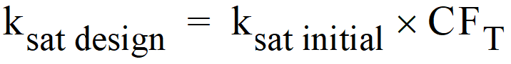
The design infiltration rate is calculated by multiplying the initial Ksat by the total correction factor.
A.2.4.1.1 Site variability and number of locations tested (CFv)
The number of locations tested must be capable of producing a picture of the subsurface conditions that fully represents the conditions throughout the facility site. The partial correction factor used for this issue depends on the level of uncertainty that adverse subsurface conditions may occur. If the range of uncertainty is low - for example, conditions are known to be uniform through previous exploration and site geological factors - one pilot infiltration test (or grain size analysis location) may be adequate to justify a partial correction factor at the high end of the range.
If the level of uncertainty is high, a partial correction factor near the low end of the range may be appropriate. This might be the case where the site conditions are highly variable due to conditions such as a deposit of ancient landslide debris, or buried stream channels. In these cases, even with many explorations and several pilot infiltration tests (or several grain size test locations), the level of uncertainty may still be high.
A partial correction factor near the low end of the range could be assigned where conditions have a more typical variability, but few explorations and only one pilot infiltration test (or one grain size analysis location) is conducted. That is, the number of explorations and tests conducted do not match the degree of site variability anticipated.
A.2.4.1.2 Uncertainty of Test Method (CFt)
This correction factor accounts for uncertainties in the testing methods. These values are intended to represent the difference in each test’s ability to estimate the actual saturated hydraulic conductivity. The assumption is the larger the scale of the test, the more reliable the result.
A.2.4.1.3 Siltation and Biofouling (CFm)
Even with a presettling basin or a basic treatment facility for pretreatment, the soil’s initial infiltration rate will gradually decline as more and more stormwater, with some amount of suspended material, passes through the soil profile. The maintenance schedule calls for removing sediment when the facility is infiltrating at only 90% of its design capacity. Therefore, a correction factor, CFm, of 0.9 is called for.
This detailed approach was obtained from (Massman, 2003).
Using the detailed approach, estimate the design (long-term) infiltration rate as follows:
Use any of the three options above, or other method approved by the local jurisdiction (as appropriate for the site) to estimate the initial Ksat.
Calculate the steady state hydraulic gradient as follows:
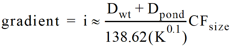
Dwt is the depth from the base of the infiltration facility to the water table in feet,
K is the initial saturated hydraulic conductivity in feet/day,
Dpond is one quarter of the maximum depth of water in the facility in feet (see Massmann et. al., 2003, for development of this equation), and
CFsize is the correction for the pond size. The correction factor was developed for ponds with bottom areas between 0.6 and 6 acres in size. For small ponds (ponds with area equal to 2/3 acre), the correction factor is equal to 1.0. For large ponds (ponds with area equal to 6 acres), the correction factor is 0.2.
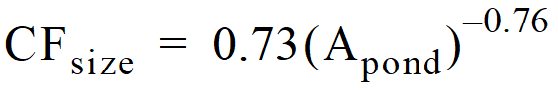
Apond is the area of pond bottom in acres.
This equation generally will result in a calculated steady state hydraulic gradient of less than 1.0 for moderate to shallow groundwater depths (or to a low permeability layer) below the BMP, and conservatively accounts for the development of a groundwater mound. A more detailed groundwater mounding analysis using a program such a MODFLOW will usually result in a gradient that is equal to or greater than the gradient calculated using the equation above.
If the calculated steady state hydraulic is greater than 1.0, the water table is considered to be deep, and a maximum gradient of 1.0 must be used. Typically, a depth to groundwater of 100 feet or more is required to obtain a gradient of 1.0 or more using this equation.
Since the gradient is a function of depth of water in the BMP, the gradient will vary as the pond fills during the season. The gradient could be calculated as part of the stage discharge calculation used in continuous runoff modeling software. As of the date of this update, no Ecology approved continuous runoff models have that capability. However, updates to those models may incorporate the capability. Until that time, calculate the steady-state hydraulic gradient using the equation above assuming a ponded depth of ¼ of the maximum ponded depth - as measured from the pond floor to the overflow.
Calculate the preliminary design infiltration rate using Darcy’s law as follows:
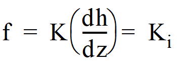
f is the preliminary design infiltration rate of water through a unit cross-section of the infiltration BMP (L/t),
K is the initial saturated hydraulic conductivity (L/t),
dh/dz is the hydraulic gradient (L/L), and
“i” is the gradient (as calcualted in Step 2 above).
Adjust the preliminary design infiltration rate to determine the design (long term) infiltration rate:
This step adjusts the preliminary design infiltration rate (as determined in Step 3 above) for the effect of a pond aspect ratio by multiplying the preliminary design infiltration rate by the aspect ratio correction factor CFaspect as shown in the following equation:
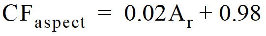
Ar is the aspect ratio for the pond (length/width of the bottom area).
In no case shall CFaspect be greater than 1.4.
The final design (long-term) infiltration rate will therefore be as follows:
Final design (long-term) infiltration rate = Ksat * i * CFaspect